Simple Atmospheric Scattering Shader

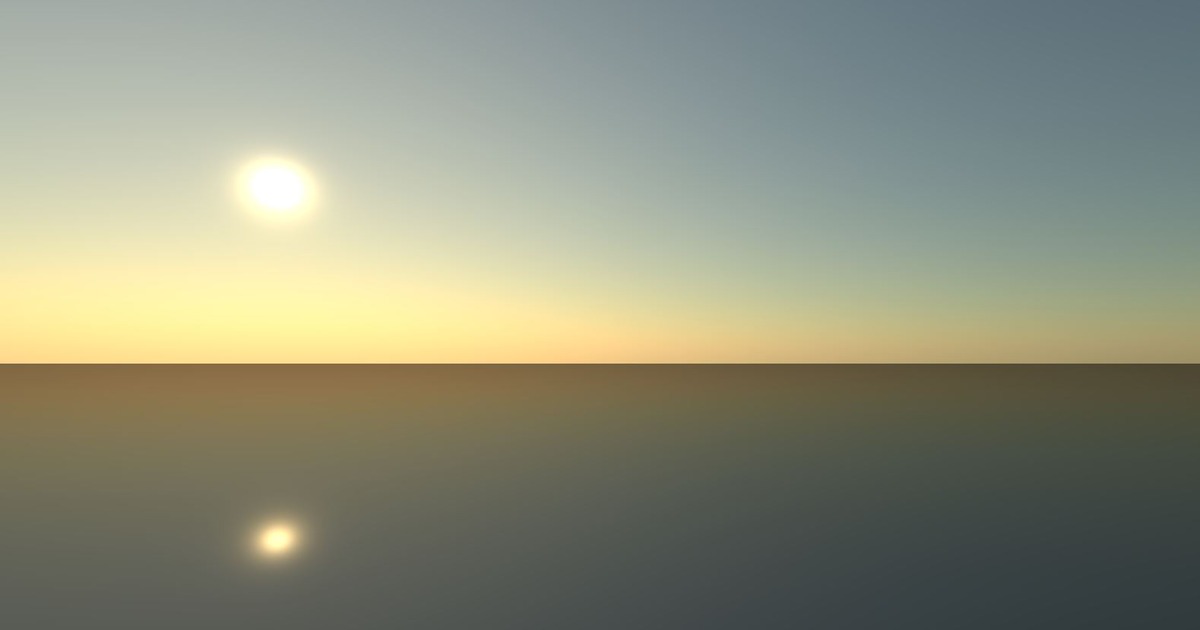
Our goal in this article is to create a simple sky texture that updates realistically as the position of the sun changes. To do this we will write a light scattering shader that will output a color given the sunlight direction and our viewing direction. Typically volumetric scattering techniques like this require ray marching through the volume in a loop, taking samples. By making some assumptions we can simplify the equations to eliminate the need to sample at all.

Atmospheric Scattering Equations

Scattering occurs when light interacts with specific particles in the atmosphere and some of its radiation is dispersed in all directions. We will use the following equations to derive the shader.

The intensity of radiation scattered at point $x$ by an angle $\theta$ is given by the Scattering Equation.

\[\begin{equation}\label{eq:1} I_S\left(x, \theta\right) \ = \ I\left(x\right) \, \sigma \ \rho \left(x\right) \phi\left(\theta\right) \end{equation}\]

Where

• $I\left(x\right)$ is the intensity at point $x$ before scattering.

• $\sigma = \left(r, g, b\right)$ is the scattering constant vector which controls how much red, green, and blue light is scattered independently.

• $\rho \left(x\right)$ is the particle density of the atmosphere at point $x$. This means if there are more particles, more light will be scattered.

• $\phi\left(\theta\right)$ is the phase function describing the distribution of scattered intensity over all directions.

This equation is not completely accurate as it is missing a constant term. However the parameter $\sigma$ will be a variable input to our shader and so it can absorb this constant.

Next we want an equation for how much intensity a light ray loses due to scattering (in any direction) over a certain distance. Integrating over $\theta$ causes the phase function to disappear (as it is a distribution function) leaving $\sigma\,\rho(x)$, the total reduction in intensity due to scattering at $x$. This is the attenuation coefficient of light through the atmosphere. We can integrate it along a path ($x_1 \to x_2$) to give the Optical Depth ($\tau$).

\[\begin{equation}\label{eq:2} \tau = \int_{x_1}^{x_2}\sigma\, \rho(x)\, dx \end{equation}\]

The resulting intensity of the ray at the end of the path ($x_1 \to x_2$) is given by the Beer-Lambert Law.

\[\begin{equation}\label{eq:3} I\left(x_2\right) = I\left(x_1\right)\ e^{-\tau} \end{equation}\]

Finally, the density of particles in the atmosphere ($\rho$) is approximated by this equation.

\[\begin{equation}\label{eq:4} \rho\left( h \right) = \,e^{-h} \end{equation}\]

Where $h$ is the altitude (height above sea level).

Again, there should be a constant for the density at sea level ($h$=0), but since the density is multiplied by $\sigma$ it can also absorb this constant. Additionally a height scale term is normally included in the exponent to control how quickly the density decays with altitude. But it turns out that in our simplified model this has exactly the same effect as the constant density at sea level and so will also be left out for simplicity.

If you would like a more rigorous approach to the equations above in the context of computer graphics, I recommend this tutorial by Alan Zucconi and this GPU Gems post.

Assumptions

We assume the following simplifications to allow us to end up with an analytical expression and avoid numerical integration.

1. Single scattering: In reality, light rays scatter around the atmosphere many times before reaching the observer. We will only consider the contribution of rays that scatter a single time into the viewing direction.

2. Parallel Sun rays: The Sun is so far away that we can safely assume that all direct Sun rays in the atmosphere travel in the same direction.

3. Flat Earth: If we assume the ground is a flat plane, then the altitude ($h$) for a position ($x$) will simply be the $y$ component, $x_y$. This is not the case for the height above the surface of a sphere and so this assumption will simplify things.

4. Infinite atmosphere: We will assume the Earths atmosphere extends infinitely above the ground and that the Sun rays travel from infinitely far away. The atmospheric density decays exponentially so it’s contribution beyond a certain point will be minimal.

Single Ray Contribution

Firstly lets consider the single ray path in this diagram.

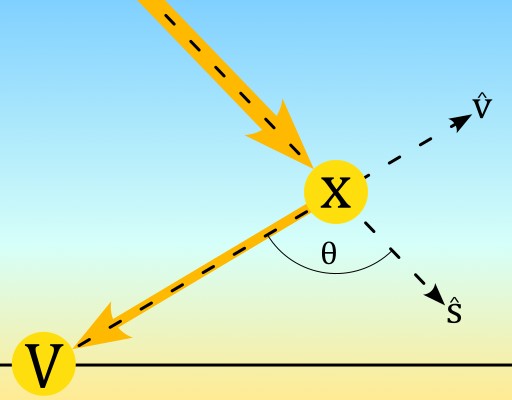Path of a single sun ray through the atmosphere

The unit vectors $\hat{s}$ and $\hat{v}$ represent the sunlight direction and viewing direction respectively.

\[\hat{s} = (s_x, s_y, s_z) \qquad \text{and} \qquad \hat{v} = (v_x, v_y, v_z)\]

The ray

• Travels from the Sun (with intensity $I_0$), along $\hat{s}$ to point $x$.
• Scatters at point $x$ by angle $\theta$.
• Travels from point $x$, along $-\hat{v}$ to the viewer at point $V$.

The ray loses intensity due to scattering along the paths from the Sun to $x$, and from $x$ to $V$. This is called Out-Scattering. The intensity of light scattered down the viewing direction contributes to the overall intensity at the viewer $V$. This is called In-Scattering.

To calculate the out-scattering along $\hat{s}$ we need to find its Optical Depth ($\tau_s$). Consider a variable $r$ that is 0 at point $x$ and increases to infinity, backwards along $\hat{s}$. Then we can write the optical depth as

\[\tau_s = \sigma\int_{0}^{\infty}\rho(-s_yr + x_y)\, dr\]

Substituting $h = -s_yr + x_y$ into the integral and evaluating gives

\[\tau_s \ = \ -\frac{\sigma}{s_y}\int_{x_y}^{\infty}\,e^{-h}\, dh \ = \ -\frac{\sigma}{s_y} \, e^{-x_y}\]

So the intensity before scattering at $x$ is

\[\begin{equation}\label{eq:5} I\left(x\right) = I_0\ \text{exp}\left(\frac{\sigma}{s_y} \, e^{-x_y}\right) \end{equation}\]

Then we can use the Scattering Equation to get the intensity after in-scattering at $x$.

\[\begin{equation}\label{eq:6} I_S\left(x\right) \ = \ I\left(x\right) \, \sigma \, \text{exp}\left(-x_y\right) \phi\left(\theta\right) \end{equation}\]

Finally, to calculate the out-scattering along the viewing direction $\hat{v}$ we need to find its Optical Depth ($\tau_v$). We can follow the same procedure as for $\tau_s$ to get

\[\tau_v \ = \ \frac{\sigma}{v_y} \, \left(1 - e^{-x_y}\right)\]

And then the resulting intensity at V, as a function of x is

\[\begin{equation}\label{eq:7} I_V\left(x\right) = I_S\left(x\right)\ \text{exp}\left(-\frac{\sigma}{v_y} \, \left(1 - e^{-x_y}\right)\right) \end{equation}\]

We can combine equations \eqref{eq:5} \eqref{eq:6}, and \eqref{eq:7} to get an expression for the light intensity at V in terms of the intensity of the Sun ray $I_0$. Terms that don’t depend on $x$ have been swept into the constants $A$ and $B$ for clarity.

\[\begin{equation}\label{eq:8} I_V\left(x\right) = I_0 \, A \, \text{exp}\left\{B \, e^{-x_y}-x_y\right\} \end{equation}\]

where

\[A = \sigma \left(1 + \text{cos}^{2}\theta \right) \text{exp}\left(-\frac{\sigma}{v_y}\right) \qquad \text{and} \qquad B = \frac{\sigma \left(v_y + s_y\right)}{v_y s_y}\]

Multiple Ray Contribution

Equation \eqref{eq:8} is the intensity contribution at $V$ for a ray scattered at $x$. We want to sum the contributions of all rays that scatter down the viewing ray, $\hat{v}$, to get the final intensity $I_V$.

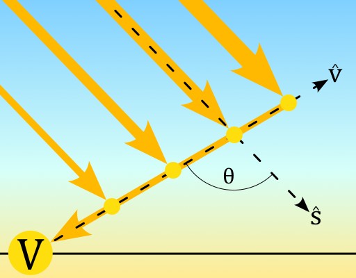Path of multiple sun rays scattered towards the viewer

Doing the same substitution trick as for the Optical Depth calculations of $\tau_s$ and $\tau_v$ we get that

\[I_V = \int_{0}^{\infty}I_V\left(v_y \, r\right) dr \ = \ I_0 \frac{A}{v_y}\int_{0}^{\infty}\text{exp}\left(B \, e^{-h}-h\right)dh\]

Now for the key step. If we had made some more physically realistic assumptions, this integral would not have an analytic solution and we would need to evaluate it numerically. But luckily, we have a pleasant substitution, $u = B \, e^{-h}$. The integral then becomes

\[\int -\frac{e^{u}}{B} \, du = -\frac{1}{B}\text{exp}\left(B \, e^{-h}\right)\]

Plugging in the limits we get

\[I_V = I_0 \, \frac{A}{Bv_y} \left(e^{B} - 1\right)\]

And replacing the constants, many terms cancel out to give our final equation.

\[\begin{equation}\label{eq:9} I_V = I_0 \, \frac{s_y}{s_y + v_y} \, \phi\left(\theta\right) \left[\text{exp}\left(\frac{\sigma}{s_y}\right) - \text{exp}\left(-\frac{\sigma}{v_y}\right)\right] \end{equation}\]

Rayleigh Scattering

Equation \eqref{eq:9} holds for a general scattering process with coefficient $\sigma$ and phase function $\phi$. Rayleigh scattering is caused by tiny particles in the atmosphere and is responsible for the blue color of the sky during the day and the orange color of the horizon when the Sun is setting. The Rayleigh coefficient $\sigma_R$ is inversely proportional to the fourth power of the light’s wavelength. We will use the following values for red, green, and blue light (which average to 1).

\[\sigma_R = S_R \, \left(0.33, 0.78, 1.89\right)\]

Where $S_R$ will allow us to control the magnitude of Rayleigh scattering. Note that blue light is scattered the most and red light the least.

The Rayleigh phase function is given by

\[\phi_R = \frac{3}{16\pi}\left(1 + \text{cos}^{2}\theta\right)\]

Note that the scattering angle $\theta$ is the angle between the sunlight direction and negative the viewing direction. So we can write $\text{cos}\theta$ as

\[\text{cos}\theta = -\hat{s} \cdot \hat{v}\]

Here is equation \eqref{eq:9} implemented in GLSL with the Rayleigh coefficient and phase function. The shader result is shown below.

const float I0 = 11.0;
const vec3 sigma_r = vec3(0.33, 0.78, 1.89);
const float S_r = 0.17;

vec3 sky_rayleigh(vec3 vd, vec3 sd) {
    return I0 * sd.y / (sd.y + vd.y) * 0.06 * (1.0 + dot(vd, sd) * dot(vd, sd)) * 
           (exp(S_r * sigma_r / sd.y) - exp(-S_r * sigma_r / vd.y));
}

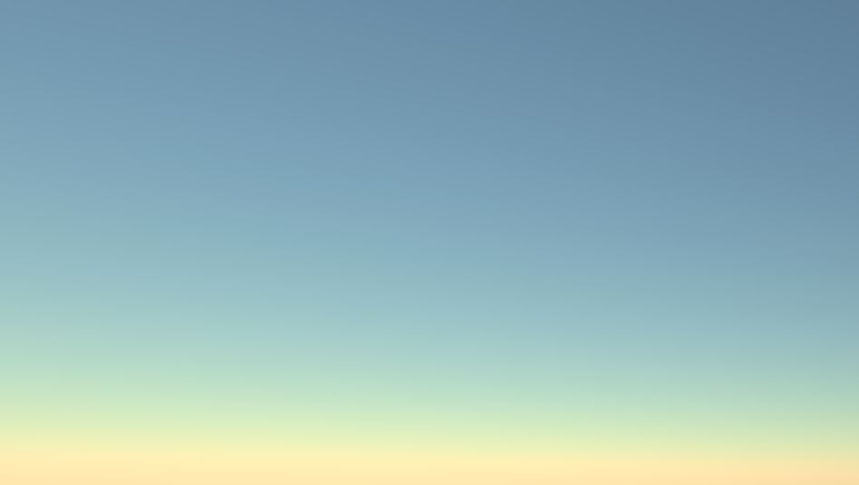Rayleigh Scattering shader result

Mie Scattering

Rayleigh scattering has given us a blue sky and yellowish horizon, but it is not particularly exciting on its own, so lets add another type. Mie scattering is caused by larger (aerosol) particles and is wavelength independent (red, green, and blue light is scattered the same amount). It causes the region of sky closer to the Sun to appear brighter.

Lets extend equation \eqref{eq:9} to allow for multiple different sources of scattering. We can redo all the steps we did before to come to the following equation.

\[\begin{equation}\label{eq:10} I_V = I_0 \, \frac{s_y}{s_y + v_y} \, \frac{\phi_{sum}}{\sigma_{sum}} \, \left[\text{exp}\left(\frac{\sigma_{sum}}{s_y}\right) - \text{exp}\left(-\frac{\sigma_{sum}}{v_y}\right)\right] \end{equation}\]

Where

\[\sigma_{sum} = \sum_{i=0}^{n}S_i\sigma_i \qquad\text{and}\qquad \phi_{sum} = \sum_{i=0}^{n}S_i\sigma_i\phi_i(\theta)\]

Here the $\sigma_i$ are normalized such that the components have an average of 1, and $S_i$ can scale the coefficient. Since Mie scattering is wavelength independent we can ignore its $\sigma$ term and just focus on the phase function $\phi$. We will use the following equation for the Mie phase function ($\phi_M$).

\[\phi_M = C \, \left(\frac{w}{1 + w - \text{cos}\theta}\right)^{2}\]

Where the parameter $w$ controls the spread of the scattered light and $C$ is a normalization constant ensuring the phase volume integrates to one. Here is a comparison of our Mie phase function with the Rayleigh phase function.

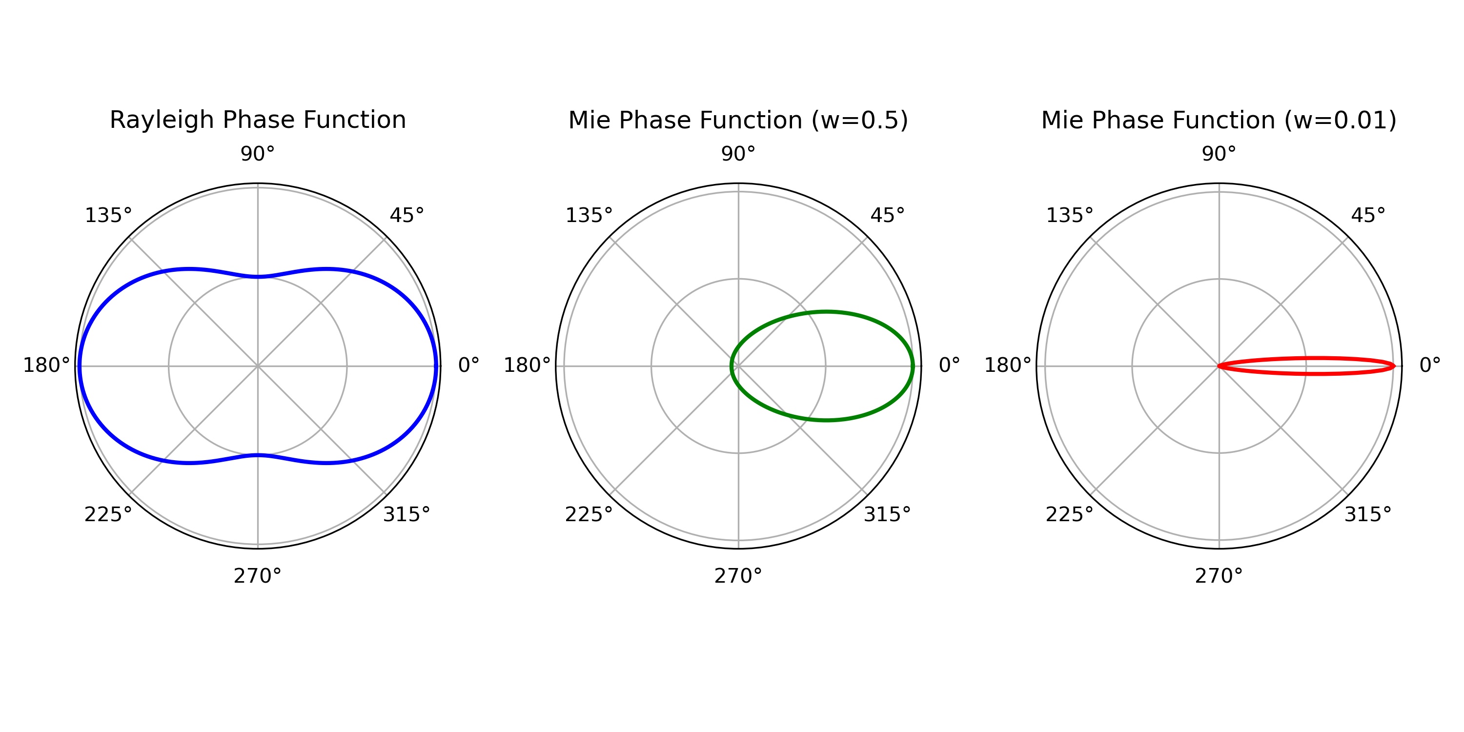Phase functions

Note that the Mie effect tends to scatter light forward (redirect only slightly) whereas the Rayleigh effect scatters light both forward and backwards symmetrically.

Rendering the Sun

To finish off the shader we will add a Sun to the sky. We will not use physically based methods to render it though. We will just use the techniques already outlined in this article to create something that looks reasonable.

Note that in our current shader we don’t consider Sun rays that reach the viewer without scattering at all. This would only happen for the view direction that lines up perfectly with the sunlight direction and so would only be represented by an infinitesimal point. To display the Sun we want to add a lot of intensity to directions that are close to parallel with the sunlight direction. However a hard cut off would not look realistic, so we want to soften the intensity as we move way from the Suns direction. Notice that a Mie scattering effect with a very low $w$ parameter does exactly that. We will add it to our shader, but only in the $\phi_{sum}$ part. If it was included in the out-scattering part it would remove too much light from the rest of the scene.

Here is the full GLSL function with Rayleigh, Mie and Sun scattering effects. The initial intensity ($I_0$) and the magnitude coefficients ($S$) were tweaked to produce pleasing results.

const float I0 = 11.0;
const vec3 sigma_r = vec3(0.33, 0.78, 1.89);
const float S_r = 0.17;
const float S_m = 0.05;
const float S_s = 0.07;
const float mie_w = 0.25;
const float sun_w = 0.0002;

vec3 sky_full(vec3 vd, vec3 sd) {

    float phase_r = 0.06 * (1.0 + dot(vd, sd) * dot(vd, sd));
    float phase_m = mie_w / (1.0 + mie_w + dot(vd, sd));
    phase_m = 0.3 * phase_m * phase_m;
    float phase_s = sun_w / (1.0 + sun_w + dot(vd, sd));
    phase_s = 4.0 * phase_s * phase_s;
    
    vec3 sigma_sum = S_r * sigma_r + S_m;
    vec3 phase_sum = S_r * sigma_r * phase_r + S_m * phase_m + S_s * phase_s;
    
    return I0 * sd.y / (sd.y + vd.y) * (phase_sum / sigma_sum) * 
           (exp(sigma_sum / sd.y) - exp(-sigma_sum / vd.y));
}

And finally here is the completed shader. Click on the title of the shader to view the source code and play around with the parameters.